Instruction Tuning Llama
In this article, we’ll fine-tune it using the Alpaca dataset we previously prepared.
This codebase and article aim to be pedagogical and straightforward. The main goal here is to understand what is happening under the hood when you fine-tune an LLM for instruction tuning.
There are more sophisticated training recipes out there like the Hugging Face transformers’ Trainer, trl, Axolotl, Peft, llama_recipes, the alignement_handbook, etc. In this article, we will try our best to make it is as simple as possible and make the training loop straightforward to follow.
NOTE: The code associate with this post can be found here.

(the left one looks more Guanaco to me but that might be a personal thing)
Downloading the Preprocessed Dataset from W&B
Let’s get started. In the previous article, we saved our preprocessed dataset as a Weights & Biases Artifact, so we can easily retrieve the dataset from there. Here’s the code:
import wandb
from pathlib import Path

run = wandb.init(project="alpaca_ft")
artifact = run.use_artifact('capecape/alpaca_ft/packed_alpaca:v0', type='dataset')
artifact_dir = Path(artifact.download())
import json

def load_jsonl(filename):
    data = []
    with open(filename, 'r') as file:
        for line in file:
            data.append(json.loads(line))
    return data

train_ds_packed = load_jsonl(artifact_dir/"train_packed_alpaca.jsonl")
eval_ds_packed = load_jsonl(artifact_dir/"eval_packed_alpaca.jsonl")
Loading Local JSON Data from Disk Using HuggingFace Datasets
Consider leveraging the Hugging Face datasets library as a more efficient container for your dataset compared to plain JSON. This option offers numerous benefits, including rapid loading, integrated map/filter functionalities, and bucket streaming, among others. Easily transform the JSONL files we generated into the datasets format utilizing the load_from_disk method.
import wandb
from datasets import load_from_disk # for some reason load_dataset gives an error

run = wandb.init(project="alpaca_ft")
artifact = run.use_artifact('capecape/alpaca_ft/packed_alpaca_hf:v0', type='dataset')
artifact_dir = artifact.download()
ds_packed = load_from_disk(artifact_dir)

# we are back where we started!
train_ds_packed = ds_packed["train"]
eval_ds_packed  = ds_packed["eval"]
max_seq_len = artifact.metadata["max_seq_len"]
DataLoader
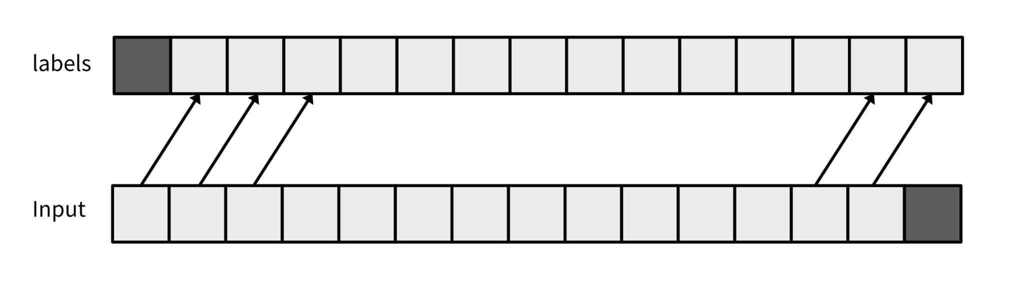
{"input_ids": input_ids[:-1], "labels": input_ids[1:]} # you actually drop one value
Please be aware that the Hugging Face model automatically handles this process for you when computing the loss on the ModelOutput.loss attribute. In this scenario, both inputs and labels are identical.
We can now put together a standard PyTorch DataLoader:
from torch.utils.data import DataLoader
from transformers import default_data_collator

batch_size = 8  # I have an A100 GPU with 40GB of RAM 😎

train_dataloader = DataLoader(
    train_ds_packed,
    batch_size=batch_size,
    collate_fn=default_data_collator, # we don't need any special collator 😎
)

eval_dataloader = DataLoader(
    eval_ds_packed,
    batch_size=batch_size,
    collate_fn=default_data_collator,
    shuffle=False,
)
b = next(iter(train_dataloader))
b.keys(), b["input_ids"][0][:25], b["labels"][0][:25]

>> (dict_keys(['input_ids', 'labels']),
 tensor([    1, 13866,   338,   385, 15278,   393, 16612,   263,  3414, 29889,
         14350,   263,  2933,   393,  7128,  2486,  1614,  2167,   278,  2009,
         29889,    13,    13,  2277, 29937]),
 tensor([13866,   338,   385, 15278,   393, 16612,   263,  3414, 29889, 14350,
           263,  2933,   393,  7128,  2486,  1614,  2167,   278,  2009, 29889,
            13,    13,  2277, 29937,  2799])) ### <<< ----  shifted by 1

# input_ids.shape: (8, 1024), labels.shape: (8, 1024)
Training Loop
We’ll initiate the training of a model by having it naively complete the sentence. As an exercise, I’ll implement this using pure PyTorch, avoiding any abstractions besides fetching the pre-trained model from the HuggingFace Hub.
I prefer storing configuration hyperparameters in a SimpleNamespace. It functions similarly to a dictionary but allows for access using dot notation. This way, I can access my batch size by referencing config.batch_size instead of config["batch_size"].
To achieve our goals, we’ll implement the following strategies:
- Train a subset of the model parameters instead of the full model.
- Utilize gradient checkpointing to conserve GPU memory. This technique involves selectively discarding and recalculating certain layers’ activations during backward passes, trading increased computation time for reduced memory usage.
- Implement Automatic Mixed Precision (AMP), which accelerates training by performing computations in half-precision (float16 or bfloat16). You can find more information about this technique here.
- Incorporate an evaluation step to sample from the model regularly.
Let’s get started!
from types import SimpleNamespace

gradient_accumulation_steps = 32 // batch_size

config = SimpleNamespace(
    model_id='meta-llama/Llama-2-7b-hf',
    dataset_name="alpaca-gpt4",
    precision="bf16",  # faster and better than fp16, requires new GPUs
    n_freeze=24,  # How many layers we don't train, LLama 7B has 32.
    lr=2e-4,
    n_eval_samples=10, # How many samples to generate on validation
    max_seq_len=max_seq_len, # Length of the sequences to pack
    epochs=3,  # we do 3 pasess over the dataset.
    gradient_accumulation_steps=gradient_accumulation_steps,  # evey how many iterations we update the gradients, simulates larger batch sizes
    batch_size=batch_size,  # what my GPU can handle, depends on how many layers are we training
    log_model=False,  # upload the model to W&B?
    mom=0.9, # optim param
    gradient_checkpointing = True,  # saves even more memory
    freeze_embed = True,  # why train this? let's keep them frozen ❄️
)

config.total_train_steps = config.epochs * len(train_dataloader) // config.gradient_accumulation_steps
model = AutoModelForCausalLM.from_pretrained(
    config.model_id,
    device_map=0,
    trust_remote_code=True,
    low_cpu_mem_usage=True,
    torch_dtype=torch.bfloat16,
    use_cache=False,
)
Freezing the Model to Save Memory: 🥶 Jeremy Howard Style
Training the full models can be computationally expensive. However, if you have a GPU capable of accommodating the entire model, you can skip this step. Instead, we’ll opt to train a subset of the model parameters, a technique pioneered by Jeremy and Seb Ruder and proven effective in various domains.
Transformer-based models like Llama consist of a stack of identical layers with a classification layer at the end. For example, Llama 2-7b comprises 32 transformer layers. In our approach, we’ll train only the last 8 layers, while you can experiment with the number of layers to freeze. It’s essential to always train the classification head, which is the last layer responsible for making predictions.
Throughout the rest of this piece, we’ll delve into techniques for training the full model efficiently, leveraging methods like LoRA for parameter fine-tuning.
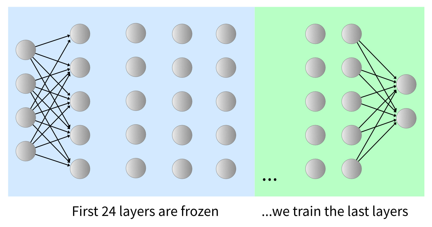
Before delving into sophisticated parameter-efficient methods, let’s adopt Jeremy Howard’s approach and freeze most of the model layers. Upon loading the model, we’ll freeze the majority of it. This strategy conserves a significant amount of memory by avoiding gradient computation on the frozen layers.
n_freeze = 24. # you can play with this parameter

# freeze layers (disable gradients)
for param in model.parameters(): param.requires_grad = False
for param in model.lm_head.parameters(): param.requires_grad = True
for param in model.model.layers[n_freeze:].parameters(): param.requires_grad = True

>> Total params: 6738.42M, Trainable: 1750.14M
# Just freeze embeddings for small memory decrease
if config.freeze_embed:
    model.model.embed_tokens.weight.requires_grad_(False);
# save more memory
if config.gradient_checkpointing:
    model.gradient_checkpointing_enable(gradient_checkpointing_kwargs={"use_reentrant": False})  # <- pytorch changed this
The code is borrowed from excellent Jeremy's notebook and video
Had to fix this cell as the "use_reentrant" argument is needed to make gradients flow form the frozen embedding!
Optimizer and Scheduler
Next, we’ll configure the optimizer and scheduler for our training process. These components are crucial for instructing PyTorch on how to compute the optimization step and adjust the learning rate accordingly. While there may be more advanced techniques to explore, starting with Adam optimizer and cosine annealing learning rate schedule is a safe choice. Additionally, we’ll set up our training loop to utilize bfloat16 precision to leverage TensorCores available on modern Nvidia GPUs. For the loss function, we’ll use Cross Entropy.
from transformers import get_cosine_schedule_with_warmup

optim = torch.optim.Adam(model.parameters(), lr=config.lr, betas=(0.9,0.99), eps=1e-5)
scheduler = get_cosine_schedule_with_warmup(
    optim,
    num_training_steps=config.total_train_steps,
    num_warmup_steps=config.total_train_steps // 10,
)

def loss_fn(x, y):
    "A Flat CrossEntropy"
    return torch.nn.functional.cross_entropy(x.view(-1, x.shape[-1]), y.view(-1))
Absolutely, leveraging the scheduler from the transformer library is a convenient option since it’s readily available. Alternatively, we can implement the scheduler in Karpathy’s style if preferred. Both approaches are valid, and using the library-provided scheduler can save time and effort in implementation.
Sampling from the Model
Sure, let’s create a simple function to sample from the model periodically for visual inspection of the model’s output. We’ll wrap the model.generate method for simplicity. We can retrieve the default sampling parameters from the GenerationConfig and pass the corresponding model_id. This approach will ensure that default parameters like temperature, top p, etc., are used consistently.
from transformers import GenerationConfig
gen_config = GenerationConfig.from_pretrained(config.model_id)

def generate(prompt, max_new_tokens=100, gen_config=gen_config):
    with torch.inference_mode():
        tokenized_prompt = tokenizer(prompt, return_tensors='pt')['input_ids'].cuda()
        output = model.generate(tokenized_prompt,
                            max_new_tokens=max_new_tokens,
                            generation_config=gen_config)
    return tokenizer.decode(output[0][len(tokenized_prompt[0]):], skip_special_tokens=True)
Certainly, we’ll execute our model over the evaluation dataset at regular intervals, specifically every 1/10th of the total training steps. We’ll log the model predictions to Weights & Biases, including the relevant sampling parameters in case we decide to modify them later. This approach ensures that we can track the model’s performance and visualize its predictions throughout the training process.
def prompt_table(prompts, log=True):
    table = wandb.Table(columns=["prompt", "generation", "concat", "max_new_tokens", "temperature", "top_p"])
    for prompt in progress_bar(prompts):
        out = generate(prompt, test_config.max_new_tokens, test_config.gen_config)
        table.add_data(prompt, out, prompt+out, test_config.max_new_tokens, test_config.gen_config.temperature, test_config.gen_config.top_p)
    if log:
        wandb.log({"predictions":table})
    return table
Validation Step
Indeed, it’s crucial to perform validation during training runs to gain insight into the training progress. While you might skip this step for concise training, computing metrics on a validation dataset can provide valuable feedback. For LLMs, sampling from the model to visualize alignment with your data is also important. Here’s how we can implement a validate function:
- Iterate through the evaluation dataloader and accumulate loss and accuracy metrics.
- Log these metrics to Weights & Biases over the entire dataset.
- Sample from the model and log the generated sequences to a Weights & Biases Table.
This comprehensive validation process ensures that we monitor the model’s performance effectively and gain valuable insights into its behavior.
@torch.no_grad()
def validate():
    model.eval();
    eval_acc = Accuracy()
    for step, batch in enumerate(tqdm(eval_dataloader)):
        batch = to_gpu(batch)
        with torch.amp.autocast("cuda", dtype=torch.bfloat16):
            out = model(**batch)
            loss = loss_fn(out.logits, batch["labels"])  # you could use out.loss and not shift the dataset
        eval_acc.update(out.logits, batch["labels"])
    # we log results at the end
    wandb.log({"eval_loss": loss.item(),
               "eval_accuracy": eval_acc.compute()})
    prompt_table(eval_dataset[:config.n_eval_samples], log=True)
    model.train();
Absolutely, incorporating validation steps during training is crucial to ensure that everything is progressing smoothly, especially in short fine-tuning scenarios. Running validation periodically allows us to assess the model’s performance and detect any potential issues early on.
In this experiment, we’ll perform validation three times, specifically at the end of every epoch. Adjusting the frequency of validation depends on factors like the task at hand and the dataset size. This approach ensures that we thoroughly evaluate the model’s performance and make necessary adjustments as needed.
A Simple PyTorch Training Loop for Your LLM
This PyTorch training loop is a conventional iteration through the training data loader, with periodic evaluation at fixed intervals. It concludes by saving the model once training completes.
Key features of this training loop include:
Gradient Accumulation: This method allows for the emulation of larger batch sizes, particularly beneficial for GPUs with limited memory capacity.
Sampling and Model Checkpoint Saving: Given the rapid training pace, only one checkpoint is saved at the conclusion of training.
Token Accuracy Computation: Token accuracy serves as a superior metric compared to loss. It offers straightforward interpretation, especially in the context of classification tasks like next token prediction in Causal Language Modeling. Jeremy Howard also advocates for accuracy as the preferred metric in such scenarios.
wandb.init(project="alpaca_ft", # the project I am working on
           tags=["baseline","7b"],
           job_type="train",
           config=config) # the Hyperparameters I want to keep track of

# Training
acc = Accuracy()
model.train()
train_step = 0
pbar = tqdm(total=config.total_train_steps)
for epoch in range(config.epochs):
    for step, batch in enumerate(train_dataloader):
        batch = to_gpu(batch)
        with torch.amp.autocast("cuda", dtype=torch.bfloat16):
            out = model(**batch)
            loss = loss_fn(out.logits, batch["labels"]) / config.gradient_accumulation_steps  # you could use out.loss and not shift the dataset
            loss.backward()
        if step%config.gradient_accumulation_steps == 0:
            # we can log the metrics to W&B
            wandb.log({"train/loss": loss.item() * config.gradient_accumulation_steps,
                       "train/accuracy": acc.update(out.logits, batch["labels"]),
                       "train/learning_rate": scheduler.get_last_lr()[0],
                       "train/global_step": train_step})
            optim.step()
            scheduler.step()
            optim.zero_grad(set_to_none=True)
            train_step += 1
            pbar.update(1)
    validate()
pbar.close()
# we save the model checkpoint at the end
save_model(
	model,
	model_name=config.model_id.replace("/", "_"),
	models_folder="models/", log=config.log_model)

wandb.finish()
This trains in around 120 minutes on an A100.
The Hugging Face course offers a similar training loop implemented in pure PyTorch to train a model sourced from the Hugging Face hub.
GPT-4 based evaluation
To compare the results generated by the fine-tuned model against GPT-3.5, and to determine which model is preferred, we can use GPT-4’s reasoning capabilities. We’ll present samples generated by both models for evaluation. Then, we’ll ask GPT-4 to provide its reasoning for choosing one over the other. This evaluation technique, akin to MT Bench, allows for a comprehensive assessment of model performance based on open-ended questions and
Indeed, GPT-4 is expected to exhibit superior reasoning capabilities compared to GPT-3.5. To ensure fairness in evaluation, we shouldn’t use the same model to generate one of the responses for judgment.
However, it’s essential to acknowledge that this evaluation strategy has its limitations. Other studies have demonstrated that it may not always be consistent with permutation, where switching the answers, or even calling the model multiple times, could result in different responses due to the stochastic nature of generation.
One approach to mitigate this variability is to set up the temperature sampling parameters closer to zero, making the model more deterministic in its responses. This ensures more consistency in the generated outputs and facilitates a fairer comparison between models.
Indeed, one of the significant advantages of this approach is its efficiency in implementing LLM-based evaluation. By utilizing a powerful model like GPT-4, we can swiftly establish a baseline score. While human-based assessment is ideal, it’s also more costly and time-consuming to implement.
To enhance the evaluation process further, we can leverage OpenAI function calling to format the output of GPT-4. This formatting can include the corresponding choice made and the reasoning behind it, providing additional context and transparency to the evaluation results.
def gpt4_judge(instruction, gen1, gen2, model="gpt-4"):
    system_prompt = ("You will be presented with a choice of two possible responses for an instruction"
                     "You have to pick the best one and give a reason why.\n"
                     "The reponse should follow the instructions and use the provided context if there is some\n"
                    "If both answers are equivalent, pick the value 0")
    message = "{instruction}\n Answer 1: \n{gen1}\n Answer 2:\n{gen2}".format(instruction=instruction, gen1=gen1, gen2=gen2)
    completion = openai.chat.completions.create(
        model=model,
        messages=[{"role": "system",
                   "content": system_prompt,
                  },
                  {"role": "user",
                   "content": message,
                  },],
        function_call = {"name": "make_choice"},
        functions = [{
                "name": "make_choice",
                "description": "Select the best generation and explain why",
                "parameters": {
                    "type": "object",
                    "properties": {
                        "choice": {
                            "type": "integer",
                            "description": "the choosen alternative, zero if equivalent",
                        },
                        "argument":{
                            "type": "string",
                            "description": "Reason why the choice was made",},},},
                    "required": ["choice", "argument"],},
        ],)
    return completion
You can inspect the results in the evaluation tables below. We generated 250 completions using GPT-3.5 and asked GPT-4 to pick the best one; we also left the possibility of marking both as equally good:
- Both models are good
- Fine-tuned Llama was better
- GPT-3.5 produced better output
To enhance the robustness of our testing, we reversed the order and re-evaluated GPT-4's selections. We retained only the choices where GPT-4 consistently picked the same answer regardless of the order. Surprisingly, in 34 instances, GPT-4 switched sides. Therefore, it's important to interpret this evaluation with caution and consider the potential variability in model judgments.
Conclusion and Final Remarks
Fine-tuning a model on an instruction dataset is a specific instance of completion training. Here, the dataset is structured in a way that enables the model to learn how to follow instructions. This serves as a simple example to clarify the complexity involved in using specialized libraries for fine-tuning.
While Llama 7B is among the smaller models available, larger models may yield better results. Nonetheless, by fine-tuning the pre-trained model, we’ve successfully endowed it with instruction-following capabilities. As a result, the model now consistently responds in the specified format and generates reasonable answers.